Back to blog

Primate social networks: basics of visualization and analysis with igraph

This tutorial (which I’m just migrating from my old site) covers the basics of importing, visualizing, and analyzing social networks in R using the igraph package. As an example, I use data on primate social networks from my undergraduate honors thesis. Before we start, install and load the packages igraph and data.table (the latter is just for reading the data directly from GitHub).

# install packages
install.packages("igraph")
install.packages("data.table")

# load packages
library("igraph")
library("data.table")

Importing social network data into R

I provide two primate social networks: one for baboons (Papio papio) and one for chimpanzees (Pan troglodytes). Both networks come from field studies on grooming interactions among troop members over a period of a few months (Boese 1975; Arnold & Whiten, unpublished data). The networks are weighted and undirected, and the node labels indicate whether individuals are male or female (the chimpanzee data also indicates whether individuals are adults, but we are going to ignore that information). The data are currently in the form of adjacency matrices in *.csv files on this GitHub repo, so we can read them into R like this:

# import Papio data from GitHub
Papio.adj <- data.frame(fread('https://raw.githubusercontent.com/rgriff23/Primate_social_networks/master/data/Papio.csv'), row.names=1)

# import Pan data from GitHub
Pan.adj <- data.frame(fread('https://raw.githubusercontent.com/rgriff23/Primate_social_networks/master/data/Pan.csv'), row.names=1)

The imported *.csv data are now in dataframes. We can convert them into weighted igraph edgelists like this:

# convert Papio to edgelist
Papio.edges <- graph_from_adjacency_matrix(as.matrix(Papio.adj), mode="undirected", weighted=TRUE)

# convert Pan to edgelist
Pan.edges <- graph_from_adjacency_matrix(as.matrix(Pan.adj), mode="undirected", weighted=TRUE)

An “edgelist” is simply a matrix of two columns: one for “source” nodes and one for “sink” nodes. Each row of the edgelist matrix represents an edge in the network. Edgelists readily scale up to large sparse networks (>1000 nodes), and igraph allows you to add attributes to nodes or vertices that can then be harnessed for visualization or analysis.

Visualization

Network visualization tools in igraph are very flexible. Here, I’ll demonstrate some basic features and use them to compare sex differences in the social networks of Pan and Papio.

We’ll begin by focusing on the Papio network. Let’s look at the most basic plot with all the default settings:

plot(Papio.edges, main="Papio")

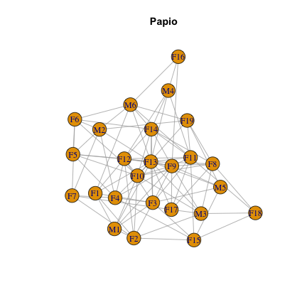
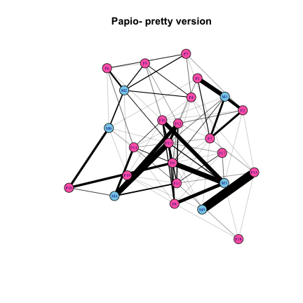
But we can do better. Let’s add colors to represent males and females, and edge weights to represent the strength of interactions among individuals. I’m going to be super gender normative and use blue for males and pink for females. In addition to coloring the vertices, I’ll make a number of other aesthetic adjustments to the graph: reduce the size of vertices and vertex labels, and color edges black:

# Define vector of colors based on sex for Papio
pap.sexes <- V(Papio.edges)$name
pap.sexes <- gsub("M[0-9]*", "skyblue", pap.sexes)
pap.sexes <- gsub("F[0-9]*", "hotpink", pap.sexes)

# Make plot
plot(Papio.edges, main="Papio- pretty version", vertex.color=pap.sexes, vertex.size=10, vertex.label.cex=0.5, edge.width=edge_attr(Papio.edges)$weight*0.25, edge.color="black")

There are many algorithms for placing nodes in the plot, some of which force the nodes into particular patterns, and others that try to spread nodes out in a meaningful, visually appealing way. The following 3 X 3 plot shows examples of many layout options available in igraph, and also illustrates how to add attributes to the graph object that will lead to automatically generated graphical parameters such as node and edge colors or weights.

# Add attributes to new network, Papio.edges2
Papio.edges2 <- set.vertex.attribute(Papio.edges, "color", value=pap.sexes)
Papio.edges2 <- set.vertex.attribute(Papio.edges2, "size", value=10)
Papio.edges2 <- set.edge.attribute(Papio.edges2, "width", value=edge_attr(Papio.edges)$weight*0.1)
Papio.edges2 <- set.edge.attribute(Papio.edges2, "color", value="black")

# Plot window
layout(matrix(1:9, 3, 3, byrow=TRUE))
par(mar=c(1,0,3,0))

# Make plots
plot(Papio.edges2, main="Grid", layout=layout_on_grid, vertex.label=NA)
plot(Papio.edges2, main="Circle", layout=layout_in_circle, vertex.label=NA)
plot(Papio.edges2, main="Sphere", layout=layout_on_sphere, vertex.label=NA)
plot(Papio.edges2, main="Simulated annealing", layout=layout_with_dh, vertex.label=NA)
plot(Papio.edges2, main="Force directed", layout=layout_with_fr, vertex.label=NA)
plot(Papio.edges2, main="Spring model", layout=layout_with_kk, vertex.label=NA)
plot(Papio.edges2, main="Multidimensional scaling", layout=layout_with_mds, vertex.label=NA)
plot(Papio.edges2, main="Randomly", layout=layout_randomly, vertex.label=NA)
plot(Papio.edges2, main="Nicely", layout=layout_nicely, vertex.label=NA)

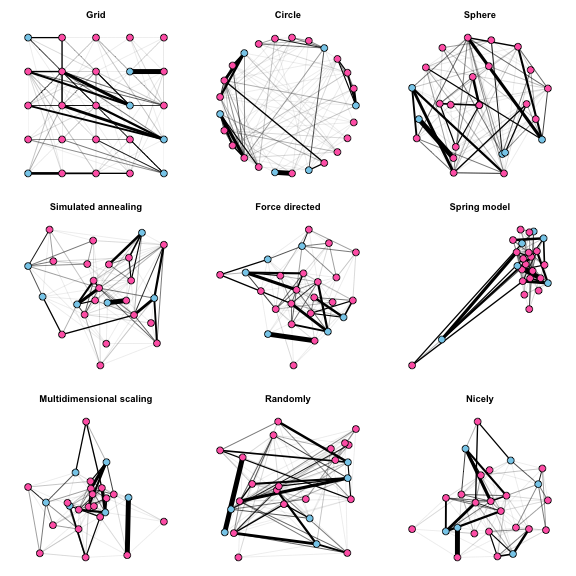
The default option is “nicely”, which will apply a force-directed layout and usually works pretty well. It attempts to do 5 things:

1. Distribute vertices evenly in the frame
2. Minimize edge crossings
3. Make edge lengths uniform
4. Reflect inherent symmetry
5. Conform to the frame

This method generally makes the nodes and edges easy to see, although a potential downside is that the initial configuration of nodes in the force-directed algorithm is random, such that subsequent plots of the same network look different.

Now, let’s do a comparison between the Pan and Papio networks (we’ll have to define the color coding for sexes for Pan):

# Define vector of colors based on sex for Pan
pan.sexes <- vertex_attr(Pan.edges)$name
pan.sexes <- gsub("[A-D]M[0-9]*", "skyblue", pan.sexes)
pan.sexes <- gsub("[A-D]F[0-9]*", "hotpink", pan.sexes)

# Add attributes to Pan network
Pan.edges2 <- set.vertex.attribute(Pan.edges, "color", value=pan.sexes)
Pan.edges2 <- set.vertex.attribute(Pan.edges2, "size", value=10)
Pan.edges2 <- set.edge.attribute(Pan.edges2, "width", value=edge_attr(Pan.edges)$weight*0.0005)
Pan.edges2 <- set.edge.attribute(Pan.edges2, "color", value="black")

# Plot window
layout(matrix(1:2, 1, 2))
par(mar=c(0,0,2,0))

# Make plots
plot(Papio.edges2, main="Papio", vertex.label=NA)
plot(Pan.edges2, main="Pan", vertex.label=NA)

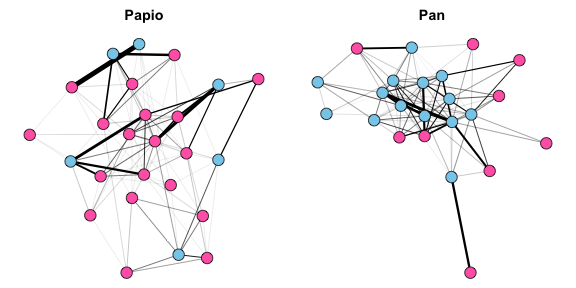
This plot reveals exactly what any primatologist would expect. The matriarchal baboons, Papio, have females at the center of the network, and females have numerous interactions with other females. Meanwhile, the relatively small number of Papio males are more peripheral, and there are few relationships between male baboons- rather, male grooming interactions are primarily with females. In contrast, the patriarchal chimpanzees, Pan, have males at the center of the network. Males chimps have many interactions among themselves, while females are peripheral and appear to interact exclusively with males rather than with each other.

Analysis

Network metrics fall into two major categories: 1) node or individual-level metrics, and 2) whole network-level metrics. Below, I briefly introduce and demonstrate how to compute some of the most common metrics used in social network analysis, and use them to make comparisons between the Pan and Papio social networks.

Individual level metrics

Individual-level metrics capture the relative “importance” of nodes in a network. There are many different metrics that have different properties, and their appropriateness depends on the research question. The simplest metric is “degree centrality”, which is defined as the number of connections for a given node.

# Compute degree
pan.degree <- degree(Pan.edges)
papio.degree <- degree(Papio.edges)

A slightly more nuanced metric is “strength centrality”, which is defined as the sum of the weights of all the connections for a given node. This is also sometimes called “weighted degree centrality”.

# Compute strength
pan.strength <- strength(Pan.edges)
papio.strength <- strength(Papio.edges)

Closeness centrality is a measure of how far other nodes are from the node in question. Nodes with high closeness centrality are likely to be relatively efficient in receiving or transmitting information to/from distant parts of the social network.

# Weighted closeness
pan.closeness <- closeness(Pan.edges)
papio.closeness <- closeness(Papio.edges)

Betweenness measures the number of shortest paths between nodes in the network that go through the node in question. Nodes with relatively high betweenness are likely to be key conduits of information flow across a network, and their removal may have a large impact on spreading phenomena.

# Weighted betweenness
pan.betweenness <- betweenness(Pan.edges)
papio.betweenness <- betweenness(Papio.edges)

Eigenvector centrality is defined as the values of the principal eigenvector for the network when represented as a matrix. Under this metric, a node’s centrality score is proportional to the centrality scores of it’s connections.

# Eigenvector centrality
pan.eigencent <- eigen_centrality(Pan.edges)
papio.eigencent <- eigen_centrality(Papio.edges)
pan.eigencent <- pan.eigencent$vector
papio.eigencent <- papio.eigencent$vector

We can now compare how these different measures of centrality differ from each other and between our two primate networks. I’m going to use the grid layout for these plots because it has a consistent structure that maximizes space between the nodes, and I am plotting node sizes proportional to their centrality scores (normalizing them so that the largest centrality score always corresponds to a node size of 30).

# Set grid layout attribute
Papio.edges3 <- set.graph.attribute(Papio.edges2, "layout", layout.grid)
Pan.edges3 <- set.graph.attribute(Pan.edges2, "layout", layout.grid)

# Plot networks with node size propotional to centrality
layout(matrix(1:10, 2, 5, byrow = TRUE))
par(mar=c(0,2,2,0))
plot(Papio.edges3, vertex.label=NA, main="Degree", vertex.size=(30*papio.degree)/max(papio.degree))
mtext("Papio", side=2)
plot(Papio.edges3, vertex.label=NA, main="Strength", vertex.size=(30*papio.strength)/max(papio.strength))
plot(Papio.edges3, vertex.label=NA, main="Closeness", vertex.size=(30*papio.closeness)/max(papio.closeness))
plot(Papio.edges3, vertex.label=NA, main="Betweenness", vertex.size=(30*papio.betweenness)/max(papio.betweenness))
plot(Papio.edges3, vertex.label=NA, main="Eigenvector Centrality", vertex.size=(30*papio.eigencent)/max(papio.eigencent))
plot(Pan.edges3, vertex.label=NA, vertex.size=(30*pan.degree)/max(pan.degree))
mtext("Pan", side=2)
plot(Pan.edges3, vertex.label=NA, vertex.size=(30*pan.strength)/max(pan.strength))
plot(Pan.edges3, vertex.label=NA, vertex.size=(30*pan.closeness)/max(pan.closeness))
plot(Pan.edges3, vertex.label=NA, vertex.size=(30*pan.betweenness)/max(pan.betweenness))
plot(Pan.edges3, vertex.label=NA, vertex.size=(30*pan.eigencent)/max(pan.eigencent))

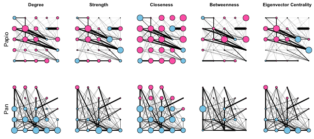
These plots show that in general, females tend to occupy more central positions in the Papio network, while males tend to occupy more central positions in the Pan network. These plots also make it clear that the different measures of centrality capture different features of network connectivity. Degree, strength, and eigenvector centrality paint fairly similar pictures of “importance” in these networks, while closeness and betweenness are very different. Closeness does not vary much across either the Pan or Papio networks, reflecting the fact that in such small, dense networks, all nodes are close to all other nodes. On the other hand, betweenness centrality identifies a small number of individuals as being important “stepping stones” connecting different individuals in the network. In particular, one male in the Pan network stands out as having the highest betweenness centrality, even though that individual does not have very high degree, strength, or eigenvector centrality.

Network level metrics

Network-level metrics aim to capture something about the structure of the overall network. These metrics are related to emergent properties of the network, such as the efficiency of information flow or the vulnerability of the network to disturbances. Most network-level metrics relate to one of two intuitive features of network structure: 1) centralization, the extent to which a small number of nodes in the network are highly influential; and 2) modularity, the extent to which the network is comprised of highly connected subunits.

Centralization

Measures of network centralization correspond to individual-level centrality measures, and basically measure the extent to which social interactions are centered on the most central node in the network. Computation of centralization metrics typically take the following steps:

1. Compute individual-level centrality measures
2. Sum the differences between the centrality score of the most central node and all other nodes
3. Normalize by dividing the sum from step 2 by the theoretical maximum sum for the maximally centralized network with the same number of nodes

There are igraph functions for computing the centralization index for all of the centrality metrics we considered in the previous section, except for strength centrality.

# Centralization scores for Papio
pap.centz <- centr_degree(Papio.edges)$centralization
pap.centz[2] <- centr_clo(Papio.edges)$centralization
pap.centz[3] <- centr_betw(Papio.edges)$centralization
pap.centz[4] <- centr_eigen(Papio.edges)$centralization

# Centralization scores for Pan
pan.centz <- centr_degree(Pan.edges)$centralization
pan.centz[2] <- centr_clo(Pan.edges)$centralization
pan.centz[3] <- centr_betw(Pan.edges)$centralization
pan.centz[4] <- centr_eigen(Pan.edges)$centralization

# Table
tab.centz <- rbind(Papio=pap.centz, Pan=pan.centz)
dimnames(tab.centz)[[2]] <- c("Degree", "Closeness", "Betweenness", "Eigenvector")
tab.centz

         Degree Closeness Betweenness Eigenvector
Papio 0.3433333 0.3494808  0.10884700   0.5372668
Pan   0.3320158 0.3870215  0.09206458   0.4410753

One can also get an idea of how centralized a network is from looking at the distribution of centrality scores. Essentially, if there are many nodes with low centrality and very few nodes with high centrality, then the network is highly centralized. Here are what the centrality distributions look like for different centrality measures on the two networks.

# Plot histograms of centrality scores
layout(matrix(1:10, 2, 5, byrow = TRUE))
par(mar=c(3,5,3,1))
hist(papio.degree, main="Degree", col="gray", xlab="", ylab="")
mtext("Papio", side=2, line=3)
hist(papio.strength, main="Strength", col="gray", xlab="", ylab="")
hist(papio.closeness, main="Closeness", col="gray", xlab="", ylab="")
hist(papio.betweenness, main="Betweenness", col="gray", xlab="", ylab="")
hist(papio.eigencent, main="Eigenvector centrality", col="gray", xlab="", ylab="")
hist(pan.degree, main="", col="gray", xlab="", ylab="")
mtext("Pan", side=2, line=3)
hist(pan.strength, main="", col="gray", xlab="", ylab="")
hist(pan.closeness, main="", col="gray", xlab="", ylab="")
hist(pan.betweenness, main="", col="gray", xlab="", ylab="")
hist(pan.eigencent, main="", col="gray", xlab="", ylab="")

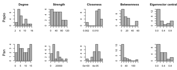
The Papio network shows moderate centralization for all metrics except closeness centrality, which is consistently high across individuals (indicating that everyone is close to everyone else, as expected in a small densely connected network). The Pan network shows moderate centralization for strength, betweenness, and eigenvector centrality, but lower centralization for degree and closeness.

Modularity

Modularity analysis can either be hypothesis driven or exploratory. Hypothesis driven modularity analysis involves testing for the significance of an a priori division of the network into modules, while exploratory modularity analysis involves applying an optimization algorithm to identify modules in a network without an a priori hypothesis.

With small, densely connected networks such as ours, I would not expect modularity to be strong. Baboon troops are united by a core group of bonded females, while chimpanzee troops are united by a core group of bonded males. However, there may be subtle subdivisions within these groups. Let’s run a clustering algorithm and see what it finds:

# Clustering algorithm for baboons
Papio.clust <- cluster_spinglass(Papio.edges)

# Clustering algorithm for chimpanzees
Pan.clust <- cluster_spinglass(Pan.edges)

We can use the output from the clustering analysis to make a nifty plot that depicts the modules in the network:

# Overlay modules on network plots
layout(matrix(1:2, 1, 2))
par(mar=c(1,1,2,1))
plot(Papio.edges2, vertex.label=NA, mark.groups=communities(Papio.clust), main="Papio")
plot(Pan.edges2, vertex.label=NA, mark.groups=communities(Pan.clust), main="Pan")

Interestingly, the Papio modules reveal a structure in which individual males tend to be associated with one or more females. Inspection of the plot reveals that there are six modules corresponding to each of the six males in the Papio group. Thus, even though the baboons form a cohesive social group, subdivisions within the group reflect a one-male unit structure.

In contrast, the Pan modules have more variable composition. There is one large module (green) composed entirely of males, another module (red) composed of several central males and over half of the females in the troop, and finally there are three small modules composed of a single male and female each. This likely reflects different mating strategies of individuals in the troop: the red module likely represents high ranking males and females that preferentially associate with them, the green all-male module likely represents younger/low ranking males with little access to females, and the three modules with pairs likely represents males pursuing a “consortship” strategy, where they focus on maintaining mating priority over a single female rather than competing with high-ranking males for access to many females.

References

• Arnold & Whiten. Unpublished data.

• Boese, G.K. (1975). “Social Behavior and Ecological Considerations of West African Baboons (Papio papio)” in Socioecology and Psychology of Primates, P. 208

• Newman, M.E.J. 2010. Networks: An Introduction. Oxford University Press.

Back to blog