BayesTraits Wrapper (btw) version 1
IMPORTANT NOTE: This is an out-of-date version of btw. For the up-to-date version (which includes Windows compatibility, support for BayesTraitsV3, and a much simpler approach to specifying BayesTraits commands), see here.
This is an R package for running BayesTraits from R (Mac OS and BayesTraits V2 only). The functions work by using system to run BayesTraits on your system and delete the output files after importing them into R.
BayesTraits was developed by Mark Pagel and Andrew Meade, and is available from their website as an executable file that can be run from a command line program such as Terminal. Consult the BayesTraits documentation before using btw.
I think there are two major advantages to using btw rather than running BayesTraits from the command line. First, if you are comfortable with R, btw makes it easy to incorporate BayesTraits into R scripts. Second, btw automatically pulls the output of btw into R in a ready-to-use format, which greatly simplifies your workflow if you want to analyze your BayesTraits output in R.
Below, I demonstrate usage of btw.
Set-up
If you have the devtools package installed, you can intall version 1 of btw from GitHub like this (note that the ref="v1" argument specifies version 1 of btw:
library(devtools)
install_github("rgriff23/btw", ref="v1")
library(btw)
Before using any of the functions that call BayesTraitsV2, you have to download Version 2 of BayesTraits. You then have to tell btw where to find it on your computer by defining the hidden variable .BayesTraitsPath. You have to do this every time you start a new R session. Be sure to specify the FULL path.
.BayesTraitsPath <- "~/Desktop/GitHub/btw/BayesTraitsV2"
The package includes some examples of tree and data files. You can load them into your R session after you load btw:
data(primates)
Some important formatting points that apply to the data for the Discrete and Continuous functions:
- Phylogenies must be of class
phyloormultiPhylo - The first column of your data file must contain species names
- Species names must match exactly between the tree and data (but order doesn’t matter)
- You cannot have spaces in your species names
- Discrete characters should be represented with characters or factors (not integers!) between 0 and 9
- A discrete character/factor with more than 1 digit is interpreted as ambiguous (e.g., “01”) indicates that the species is equally likely to be in state “0” or “1” (now you see why the discrete characters can’t be of class ‘integer’, because 01 would just be seen as 1)
- If testing for correlated evolution in discrete characters, use 0 and 1 as the character states
- The only valid way to represent missing data is with a “-“ character
Now let’s use btw to run some BayesTraits analyses.
Using Discrete in ‘Multistate’ mode
Multistate is used when you have data on a single categorical trait. An example of this sort of data is `primate.discrete1’, which contains data on trait that takes 3 discrete values (0, 1, and 2). Viewing the data reveals one missing value (Colobus_polykomos) and one ambiguous value (Hylobates_agilis).
primate.discrete1
                    species trait
  1    Cercocebus_torquatus     1
  2      Cercopithecus_mona     0
  3 Cercopithecus_nictitans     0
  4      Colobus_angolensis     1
  5         Colobus_guereza     2
  6       Colobus_polykomos     -
  7            Homo_sapiens     0
  8        Hylobates_agilis    01
More than two character states can be modeled, but keep in mind that the number of model parameters increases rapidly with the number of character states. Specifically, for n states there are $n^2$ - n rate parameters, such that by the time you get to 4 states, 12 rates must be estimated!
Let’s fit a maximum likelihood model where we allow each of the 6 rates (0->1, 1->0, 1->2, 2->1, 0->2, 2->0) to be independent, and use a likelihood ratio test to compare it to a symmetric model where all rates must be equal to each other.
asymmetric <- Discrete(primate.tree1, primate.discrete1, "ML")
symmetric <- Discrete(primate.tree1, primate.discrete1, "ML", res="q01")
lrtest(symmetric, asymmetric)
    model1.Lh model2.Lh LRstat pval
  1 -4.572531 -4.572531      0    1
The likelihood ratio test is not significant, indicating that we should favor the simpler model. In this case, the symmetric model is simpler because it only estimates one parameter, while the asymmetric model estimates six.
Reversible jump hyper-prior model
Another way to get at the question of whether there is evidence for multiple rates of evolution among the 3 character states is to run a reversible jump model, which will sample across models in proportion to their likelihood and return a distribution of model structures. We will also take phylogenetic uncertainty into account by sampling across a block of 100 trees, primate.tree100.
multirj <- Discrete(primate.tree100, primate.discrete1, "Bayesian", rj="uniform -100 100", bi=10000, it=1000000, sa=1000)
We can use the function rjmodels to get a quick summary of the models sampled in the reversible jump analysis.
rjout <- rjmodels(multirj)
rjout
  $NumModels
  [1] 406

  $TopTen

  '0 Z 0 0 0 0  '0 0 0 Z 0 0  '0 0 0 0 0 0  '0 0 0 Z Z 0  'Z 0 0 0 0 0
     0.03636364    0.02727273    0.02424242    0.01818182    0.01717172
  '0 0 0 Z 0 Z  '0 Z 0 0 0 Z  'Z 0 Z 0 0 0  '0 Z 0 0 Z 0  '0 0 0 0 1 0
     0.01616162    0.01616162    0.01616162    0.01212121    0.01010101
Output indicates that an extremely large number of models were sampled in the posterior distribution (406!) and the top ten models represented an extremely small proportion of the total sample of models (the best model represented about 4% of all the models). This indicates that support for any one model over other possible models is weak, and in light of this, the simplest model should be chosen (i.e., all rates equal).
Fossilizing and reconstructing an ancestral state
Next, let’s compare an unconstrained model to a model where we fossilize the ancestor of Homo_sapiens and Hylobates_agilis to be 2. And let’s do it in a Bayesian framework.
fossilape <- Discrete(primate.tree1, primate.discrete1, "Bayesian", fo="2 Homo_sapiens Hylobates_agilis")
nofossil <- Discrete(primate.tree1, primate.discrete1, "Bayesian")
bf <- bftest(fossilape, nofossil)
bf
    BayesFactor BetterModel
  1    2.778082     Model 2
The Bayes factor is 2.778082 and the unconstrained model is preferred. We can also estimate the probabilities of different ancestral states for the Homo_sapiens/Hylobates_agilis ancestor. Let’s use maximum likelihood this time (the default setting).
reconstruct <- Discrete(primate.tree1, primate.discrete1, mrca="Homo_sapiens Hylobates_agilis")
reconstruct
    Tree.No       Lh      q01 q02 q10      q12      q20      q21 Root.P.0.
  1       1 -4.57253 0.030713   0   0 0.230283 0.144508 0.407705  0.329525
    Root.P.1. Root.P.2. mrcaNode1.P.0. mrcaNode1.P.1. mrcaNode1.P.2.
  1  0.334345   0.33613       0.439357       0.263306       0.297338
Results indicate that there is only a 29.7% chance that the Homo_sapiens/Hylobates_agilis ancestor was in state 2, which is consistent with our finding that the model where we fossilized that ancestor at 2 was significantly worse than the unconstrained model.
Using Discrete in ‘Discrete’ mode
Discrete can be used to test for correlated evolution between a pair of binary characters. An example of this data is primate.discrete2, which contains a pair of binary traits.
Independent vs. dependent evolution test
Let’s do the significance test for correlated (i.e., dependent) evolution for the two traits in maximum likelihood mode.
nocorrD <- Discrete(primate.tree1, primate.discrete2)
corrD <- Discrete(primate.tree1, primate.discrete2, dependent=TRUE)
lrtest(corrD, nocorrD)
    model1.Lh model2.Lh   LRstat      pval
  1 -5.686009 -6.786591 2.201164 0.1379066
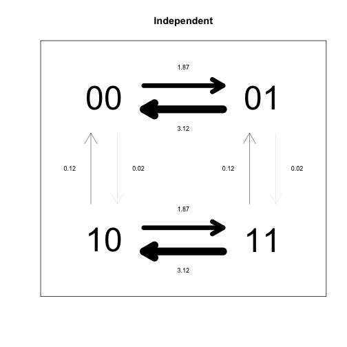
The difference is not significant, indicating that the simpler model (no correlation) should be preferred. The output from these models can be a little confusing, but the plotdiscrete function allows visualization of the results.
plotdiscrete(nocorrD, main="Independent")
plotdiscrete(corrD, main="Dependent")
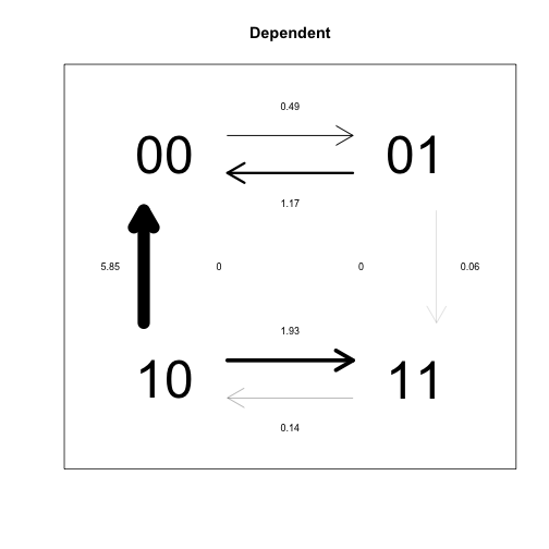
In this analysis, each pair of states for the two traits is treated as a separate state (00, 01, 10, 11). The independent model forces some pairs of rate parameters to be identical, because the idea is that transition rates for each trait should be the same, indepent of what state the other trait is in (this leads to 4 overall parameters). By contrast, the dependent model assumes that transition rates for each trait depend on the state of the other trait, such that different rates need to be estimated (leading to 8 overall parameters). Due to the different constraints imposed on the two models, their transition rate matrices look very different, but as the likelihood ratio test demonstrates, the difference is not significant.
Using Continuous
The Continuous function can be used to compare models of evolution for one or more continuous traits. The format for the data files is the same as for discrete traits.
Phylogenetic signal test
Continuous supports the estimation of several parameters that correspond to different models of evolution. Perhaps the most widely used of these is lambda, the phylogenetic signal parameter developed by Mark Pagel (1999). Let’s test the hypothesis that the maximum likelihood estimate of lambda is significantly different from 0 for a single continuous trait.
lambda0 <- Continuous(primate.tree1, primate.continuous1, lambda=0)
lambdaML <- Continuous(primate.tree1, primate.continuous1, lambda="ML")
lrtest(lambdaML, lambda0)
    model1.Lh model2.Lh LRstat pval
  1  1.115431  1.115431      0    1
The p-value is not significant, so there is no evidence that lambda is different from 0 (which corresponds to no phylogenetic signal in the data).
Correlated evolution test
We can test for a significant correlation between pairs of continuous traits. The tc parameter fixes the correlation between two traits to be 0, and this can be used as a null model to test for a significant correlation.
nocorrC <- Continuous(primate.tree1, primate.continuous2, tc=TRUE)
corrC <- Continuous(primate.tree1, primate.continuous2)
lrtest(nocorrC, corrC)
    model1.Lh model2.Lh   LRstat      pval
  1  -6.18303 -5.736392 0.893276 0.3445911
The p-value is not significant, so there is no evidence for a correlation between these traits.
Regression model
Continuous can also be used to fit regression models with 1 or more predictor variables. The first variable in the dataframe is automatically treated as the response variable. Let’s fit a regression model with two predictor variables.
glm1 <- Continuous(primate.tree1, primate.continuous3, regression=TRUE)
glm1
    Tree.No        Lh      Alpha     Beta.2   Beta.3         Var       R.2
  1       1 -3.448363 0.05771658 -0.5048425 1.243642 0.008530046 0.4391672
           SSE       SST Error.Ratio s.e..Alpha s.e..Beta.2 s.e..Beta.3
  1 0.06824037 0.1216769   0.4391672   0.344801    0.734077    0.570176
    Kappa Delta Lambda OU
  1     1     1      1  0
We can compare the standard errors of regression parameters to their estimated values to assess whether they are significant. In this model, the estimate of Beta.2 is -0.5 with a standard error of 0.73, while the estimate of Beta.3 is 1.24 with a standard error of 0.57. Thus, only Beta.3 is significantly different from 0 (because 0 lies outside the interval 1.24 +/- 0.57).
MCMC diagnostics
A convenient thing about running BayesTraits with btw is that the output from Bayesian MCMC analyses are basically ready to be analyzed with the R package coda for doing MCMC diagnostics. Here, I provide some examples of how coda can be used to do health assessments for MCMC chains. First, let’s make some data (this won’t be pretty… the point is just to see how it works).
coda.demo <- Discrete(primate.tree100, primate.discrete1, "Bayesian", it=1000000)
Now load the coda package (if it isn’t already installed, then install it!).
library(coda)
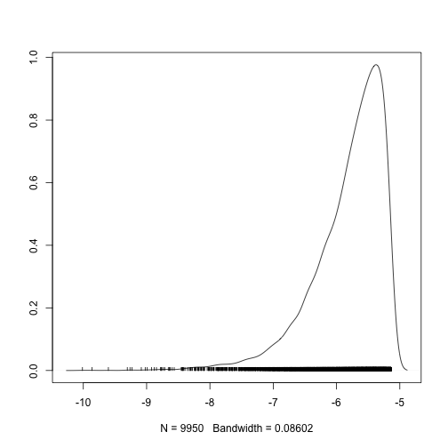
In one easy step, we can prepare the MCMC output for analysis in coda. The key is that coda functions work on objects of class mcmc, so we need to convert columns from our dataframe into mcmc objects before using coda plotting functions. We can do this by wrapping the variable we want to plot with the mcmc function.
Here is a density plot for the likelihood.
densplot(mcmc(coda.demo$Lh))
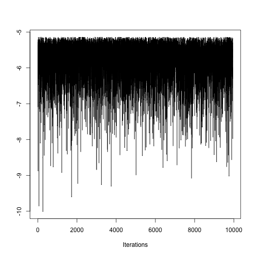
Here is a trace plot for the likelihood.
traceplot(mcmc(coda.demo$Lh))
Here is an autocorrelation plot for the likelihood.
autocorr.plot(mcmc(coda.demo$Lh))
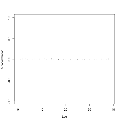
This all just goes to say that btw makes it easy for you to use the tools provided by coda to do MCMC diagnostics. Check out the coda documentation for more info!
References
Pagel, M. (1999). “Inferring the historical patterns of biological evolution.” Nature 401(6756): 877-884.
